        %%{init: { 'logLevel': 'debug', 'theme': 'base' } }%%
graph LR
    waveform[Get Data] --> correlate(Correlation)
    correlate -->|save| corrdb[(CorrDB/hdf5)]
    corrdb --> monitor
    monitor[Measure dv] -->|save| dv{{DV}}:::active
    click waveform "../trace_data.html" "trace_data"
    click correlate "../correlate.html" "correlate"
    click monitor "../monitor.html" "monitor"
    click corrdb "../corrdb.html" "CorrDB"
    click dv "../monitor/dv.html" "DV"
    classDef active fill:#f666, stroke-width:4px, stroke:#f06;
Reading and Handling of DV objects#
SeisMIC uses DV objects to handle velocity changes. Those can for example saved, loaded, and plotted.
There are also a number of processing functions and methods that use DV objects.
Read a DV Object from Disk#
Most likely, you will want to read the velocity changes that were computed in the previous step. SeisMIC uses binary npz format to
store those. You will find the files in the folder that you have defined earlier (i.e., in the yaml file).
Load the object with seismic.monitor.dv.read_dv(). It only takes one argument: the path to the dv object.
from seismic.monitor.dv import read_dv

dv = read_dv('/path/to/my/dv/DV-net0-net1.stat0-stat1.loc0-loc1.cha0-cha1.npz')

# We can also print some information about them
print(dv)
single_ref stretch velocity change estimate of X9-X9.IR1-IR1.HHE-HHE. starttdate: Mon Jan 25 00:00:00 2016 enddate: Fri Feb 5 00:00:00 2016
processed with the following parameters: {‘freq_min’: 2.0, ‘freq_max’: 4.0, ‘tw_start’: 3.5, ‘tw_len’: 8.5}
Plotting#
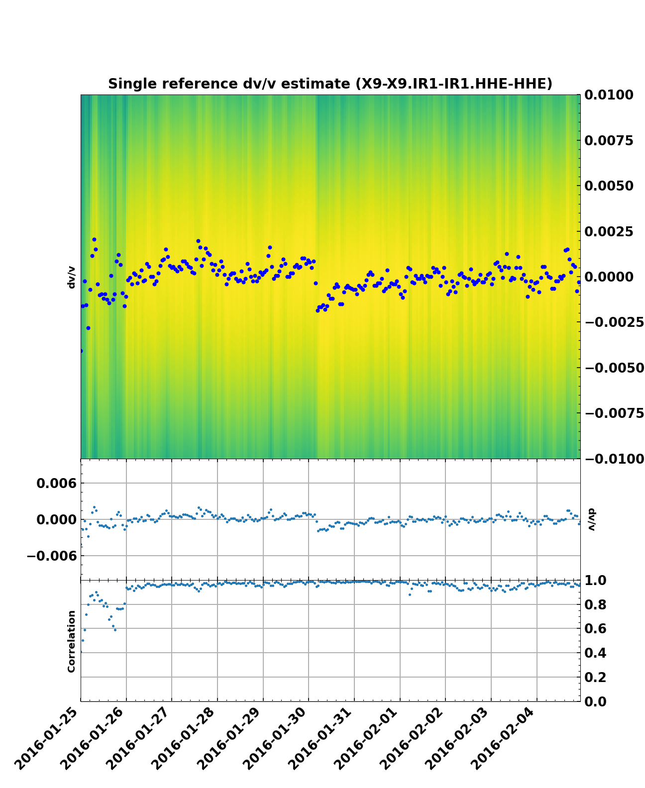
You can create a plot of the dv object with seismic.monitor.dv.DV.plot(). The result will look like this:

Stacking/Averaging Results from several stretching estimations#
As shown by Illien et al. (2023)
and Makus et al. (2023),
the similarity matrix (i.e., the result of the stretching grid search) from several
component combinations or stations can be averaged to create more robust velocity change estimates.
This is implemented in the function seismic.monitor.monitor.average_components().
Inverting Velocity Changes onto a spatial grid#
The module seismic.monitor.spatial implements the surface wave spatial inversion as proposed by Obermann et al. (2013).
In pratice, you will create one DVGrid and invert for each time t that you will want to
have a separate map of.
If you want to commit an inverse crime, the forward solution is also implemented in
forward_model(). Equally, you can compute the
model resolution using compute_resolution().
For further details and a more thorough how-to, refer to the spatial tutorial.
