SeisMIC Tutorial#
In the following, we will go through a simple example to compute a ambient noise correlations and monitor velocity changes using SeisMIC.
The source code is hosted here: SeisMIC.
The documentation, which this notebook is based upon is located here: SeisMIC Documentation.
As an exercise, we will download data from one channel of the station
X9.IR1 to investigate the coseismic velocity change caused by the
M7.2 2016 Zhupanov earthquake (see Makus et. al.,
2023). Without further ado,
we’ll dive right into it starting with data download.
1. Download the raw data#
SeisMIC uses obspy to download data from FDSN servers.
To download the data, we will use the
`seismic.trace_data.waveform.Store_Client <https://petermakus.github.io/SeisMIC/modules/API.html#seismic.trace_data.waveform.Store_Client>`__
class and its method download_waveforms_mdl().
import os

from obspy.clients.fdsn import Client
from obspy import UTCDateTime

from seismic.trace_data.waveform import Store_Client

# Get notebook path for future reference of the database:
try: ipynb_path
except NameError: ipynb_path = os.getcwd()

os.chdir(ipynb_path)

root = os.path.join(ipynb_path, 'data')
os.makedirs(root, exist_ok=True)

starttime = UTCDateTime(2016, 1, 25)
endtime = UTCDateTime(2016, 2, 5)
network = 'X9'
station = 'IR1'


c = Client('GEOFON')
sc = Store_Client(c, root, read_only=False)
sc.download_waveforms_mdl(
    starttime, endtime, clients=[c], network=network,
    station=station, location='*', channel='HHE')
[2023-08-24 10:50:29,755] - obspy.clients.fdsn.mass_downloader - INFO: Initializing FDSN client(s) for http://geofon.gfz-potsdam.de.
[2023-08-24 10:50:29,755] - obspy.clients.fdsn.mass_downloader - INFO: Initializing FDSN client(s) for http://geofon.gfz-potsdam.de.
[2023-08-24 10:50:29,757] - obspy.clients.fdsn.mass_downloader - INFO: Successfully initialized 1 client(s): http://geofon.gfz-potsdam.de.
[2023-08-24 10:50:29,757] - obspy.clients.fdsn.mass_downloader - INFO: Successfully initialized 1 client(s): http://geofon.gfz-potsdam.de.
[2023-08-24 10:50:29,758] - obspy.clients.fdsn.mass_downloader - INFO: Total acquired or preexisting stations: 0
[2023-08-24 10:50:29,758] - obspy.clients.fdsn.mass_downloader - INFO: Total acquired or preexisting stations: 0
[2023-08-24 10:50:29,759] - obspy.clients.fdsn.mass_downloader - INFO: Client 'http://geofon.gfz-potsdam.de' - Requesting unreliable availability.
[2023-08-24 10:50:29,759] - obspy.clients.fdsn.mass_downloader - INFO: Client 'http://geofon.gfz-potsdam.de' - Requesting unreliable availability.
[2023-08-24 10:50:29,906] - obspy.clients.fdsn.mass_downloader - INFO: Client 'http://geofon.gfz-potsdam.de' - Successfully requested availability (0.15 seconds)
[2023-08-24 10:50:29,906] - obspy.clients.fdsn.mass_downloader - INFO: Client 'http://geofon.gfz-potsdam.de' - Successfully requested availability (0.15 seconds)
[2023-08-24 10:50:29,909] - obspy.clients.fdsn.mass_downloader - INFO: Client 'http://geofon.gfz-potsdam.de' - Found 1 stations (1 channels).
[2023-08-24 10:50:29,909] - obspy.clients.fdsn.mass_downloader - INFO: Client 'http://geofon.gfz-potsdam.de' - Found 1 stations (1 channels).
[2023-08-24 10:50:29,911] - obspy.clients.fdsn.mass_downloader - INFO: Client 'http://geofon.gfz-potsdam.de' - Will attempt to download data from 1 stations.
[2023-08-24 10:50:29,911] - obspy.clients.fdsn.mass_downloader - INFO: Client 'http://geofon.gfz-potsdam.de' - Will attempt to download data from 1 stations.
[2023-08-24 10:50:29,913] - obspy.clients.fdsn.mass_downloader - INFO: Client 'http://geofon.gfz-potsdam.de' - Status for 11 time intervals/channels before downloading: IGNORE
[2023-08-24 10:50:29,913] - obspy.clients.fdsn.mass_downloader - INFO: Client 'http://geofon.gfz-potsdam.de' - Status for 11 time intervals/channels before downloading: IGNORE
[2023-08-24 10:50:29,915] - obspy.clients.fdsn.mass_downloader - INFO: Client 'http://geofon.gfz-potsdam.de' - No station information to download.
[2023-08-24 10:50:29,915] - obspy.clients.fdsn.mass_downloader - INFO: Client 'http://geofon.gfz-potsdam.de' - No station information to download.
[2023-08-24 10:50:29,916] - obspy.clients.fdsn.mass_downloader - INFO: ============================== Final report
[2023-08-24 10:50:29,916] - obspy.clients.fdsn.mass_downloader - INFO: ============================== Final report
[2023-08-24 10:50:29,917] - obspy.clients.fdsn.mass_downloader - INFO: 0 MiniSEED files [0.0 MB] already existed.
[2023-08-24 10:50:29,917] - obspy.clients.fdsn.mass_downloader - INFO: 0 MiniSEED files [0.0 MB] already existed.
[2023-08-24 10:50:29,918] - obspy.clients.fdsn.mass_downloader - INFO: 0 StationXML files [0.0 MB] already existed.
[2023-08-24 10:50:29,918] - obspy.clients.fdsn.mass_downloader - INFO: 0 StationXML files [0.0 MB] already existed.
[2023-08-24 10:50:29,919] - obspy.clients.fdsn.mass_downloader - INFO: Client 'http://geofon.gfz-potsdam.de' - Acquired 0 MiniSEED files [0.0 MB].
[2023-08-24 10:50:29,919] - obspy.clients.fdsn.mass_downloader - INFO: Client 'http://geofon.gfz-potsdam.de' - Acquired 0 MiniSEED files [0.0 MB].
[2023-08-24 10:50:29,920] - obspy.clients.fdsn.mass_downloader - INFO: Client 'http://geofon.gfz-potsdam.de' - Acquired 0 StationXML files [0.0 MB].
[2023-08-24 10:50:29,920] - obspy.clients.fdsn.mass_downloader - INFO: Client 'http://geofon.gfz-potsdam.de' - Acquired 0 StationXML files [0.0 MB].
[2023-08-24 10:50:29,920] - obspy.clients.fdsn.mass_downloader - INFO: Downloaded 0.0 MB in total.
[2023-08-24 10:50:29,920] - obspy.clients.fdsn.mass_downloader - INFO: Downloaded 0.0 MB in total.
Some notes about this: 1. The method download_waveforms_mdl()
expects a list of clients as input. 2. All arguments accept wildcards
If everything worked fine. This should have created a folder called
data/mseed and data/inventory. Let’s check
os.listdir('./data/')
['inventory', 'mseed']
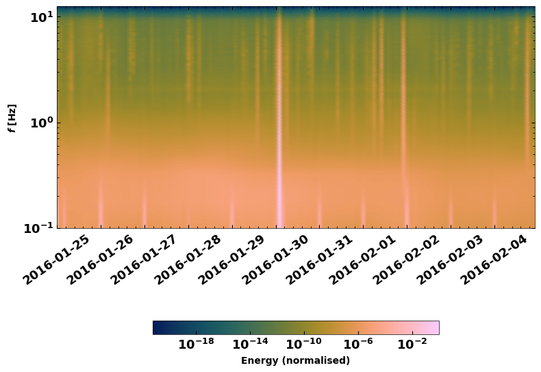
1.1 Plot a time-dependent spectrogram#
A good first step to evaluate how the noise looks in the different frequency bands is by plotting a spectral series. SeisMIC possesses an efficient implentation using Welch windows.
from seismic.plot.plot_spectrum import plot_spct_series
from matplotlib import pyplot as plt

f, t, S = sc.compute_spectrogram('X9', 'IR1', 'HHE', starttime, endtime, 7200, freq_max=12.5)
fig = plt.figure(figsize=(9, 7))
plot_spct_series(S, f, t, log_scale=True)
<Axes: ylabel='$f$ [Hz]'>
2. Compute Correlations#
That seems to have worked, so we are ready to use this raw data to compute ambient noise correlations.
2.1 Parameters#
Parameters are provided as a yaml file or a dict object. This
tutorial comes with an yaml file to process the data. Let’s have a short
look at it using bash.
!cat params.yaml
#### Project wide parameters
# lowest level project directory
proj_dir : 'data'
# Save the component combinations in separate hdf5 files
# This is faster for multi-core if True
# Set to False for compatibility with SeisMIC version < 0.4.6
save_comps_separately: True
# directory for logging information
log_subdir : 'log'
# levels:
# 'DEBUG', 'INFO', 'WARNING', 'ERROR', or 'CRITICAL'
log_level: 'WARNING'
# folder for figures
fig_subdir : 'figures'


#### parameters that are network specific
net:
    # list of stations used in the project
    # type: list of strings or string, wildcards allowed
    network : 'X9'
    station : 'IR1'

#### parameters for correlation (emperical Green's function creation)
co:
    # subdirectory of 'proj_dir' to store correlation
    # type: string
    subdir : 'corr'
    # times sequences to read for cliping or muting on stream basis
    # These should be long enough for the reference (e.g. the standard
    # deviation) to be rather independent of the parts to remove
    # type: string
    read_start : '2016-01-25 00:00:01.0'
    read_end : '2016-02-05 00:00:00.0'
    # type: float [seconds]
    # The longer the faster, but higher RAM usage.
    # Note that this is also the length of the correlation batches
    # that will be written (i.e., length that will be
    # kept in memory before writing to disk)
    read_len : 86398
    read_inc : 86400

    # New sampling rate in Hz. Note that it will try to decimate
    # if possible (i.e., there is an integer factor from the
    # native sampling_rate)
    sampling_rate : 25
    # Remove the instrument response, will take substantially more time
    remove_response : False

    # Method to combine different traces
    combination_method : 'autoComponents'

    # If you want only specific combinations to be computed enter them here
    # In the form [Net0-Net0.Stat0-Stat1]
    # This option will only be consider if combination_method == 'betweenStations'
    # Comment or set == None if not in use
    xcombinations : None

    # preprocessing of the original length time series
    # these function work on an obspy.Stream object given as first argument
    # and return an obspy.Stream object.
    preProcessing : [
                    {'function':'seismic.correlate.preprocessing_stream.detrend_st',
                    'args':{'type':'linear'}},
                    {'function':'seismic.correlate.preprocessing_stream.cos_taper_st',
                      'args':{'taper_len': 100, # seconds
                              'lossless': True}}, # lossless tapering stitches additional data to trace, tapers, and removes the tapered ends after preprocessing
                    {'function':'seismic.correlate.preprocessing_stream.stream_filter',
                      'args':{'ftype':'bandpass',
                              'filter_option':{'freqmin':0.01, #0.01
                                               'freqmax':12.49}}}
                     #{'function':'seismic.correlate.preprocessing_stream.stream_mute',
                     # 'args':{'taper_len':100,
                     #         'mute_method':'std_factor',
                     #         'mute_value':3}}
                    ]
    # subdivision of the read sequences for correlation
    # if this is set the stream processing will happen on the hourly subdivision. This has the
    # advantage that data that already exists will not need to be preprocessed again
    # On the other hand, computing a whole new database might be slower
    # Recommended to be set to True if:
    # a) You update your database and a lot of the data is already available (up to a magnitude faster)
    # b) corr_len is close to read_len
    # Is automatically set to False if you are computing a completely new db
    preprocess_subdiv: True
    # type: presence of this key
    subdivision:
        # type: float [seconds]
        corr_inc : 3600
        corr_len : 3600
        # recombine these subdivisions
        # unused at the time
        # type: boolean
        recombine_subdivision : True
        # delete
        # type: booblean
        delete_subdivision : False

    # parameters for correlation preprocessing
    # Standard functions reside in seismic.correlate.preprocessing_td and preprocessing_fd, respectively
    corr_args : {'TDpreProcessing':[
                                    {'function':'seismic.correlate.preprocessing_td.detrend',
                                    'args':{'type':'linear'}},
                                   {'function':'seismic.correlate.preprocessing_td.TDfilter',
                                   'args':{'type':'bandpass','freqmin':2,'freqmax':4}},
                                    #{'function':'seismic.correlate.preprocessing_td.mute',
                                    # 'args':{'taper_len':100.,
                                           # 'threshold':1000, absolute threshold
                                    #         'std_factor':3,
                                    #         'filter':{'type':'bandpass','freqmin':2,'freqmax':4},
                                    #         'extend_gaps':True}},
                                  #  {'function':'seismic.correlate.preprocessing_td.clip',
                                  #   'args':{'std_factor':2.5}},
                                   {'function':'seismic.correlate.preprocessing_td.signBitNormalization',
                                    'args': {}}
                                   ],
                  # Standard functions reside in seismic.correlate.preprocessing_fd
                 'FDpreProcessing':[
                                    # {'function':'seismic.correlate.preprocessing_fd.spectralWhitening',
                                    #  'args':{'joint_norm':False}},
                                    {'function':'seismic.correlate.preprocessing_fd.FDfilter',
                                     'args':{'flimit':[1.33, 2, 4, 6]}}
                                    #  {'function':seismic.correlate.preprocessing_fd.FDsignBitNormalization,
                                    # 'args':{}}
                                    ],
                 'lengthToSave':25,
                 'center_correlation':True,      # make sure zero correlation time is in the center
                 'normalize_correlation':True,
                 'combinations':[]
                }


#### parameters for the estimation of time differences
dv:
    # subfolder for storage of time difference results
    subdir : 'vel_change'

    # Plotting
    plot_vel_change : True

    ### Definition of calender time windows for the time difference measurements
    start_date : '2016-01-25 00:00:00.0'   # %Y-%m-%dT%H:%M:%S.%fZ'
    end_date : '2016-02-05 00:00:00.0'
    win_len : 3600                         # length of window in which EGFs are stacked
    date_inc : 3600                        # increment of measurements

    ### Frequencies
    freq_min : 2
    freq_max : 4

    ### Definition of lapse time window
    tw_start : 3.5     # lapse time of first sample [s]
    tw_len : 8.5       # length of window [s] Can be None if the whole (rest) of the coda should be used
    sides : 'both'   # options are left (for acausal), right (causal), both, or single (for active source experiments where the first sample is the trigger time)
    compute_tt : False  # Computes the travel time and adds it to tw_start (tt is 0 if not xstations). If true a rayleigh wave velocity has to be provided
    rayleigh_wave_velocity : 1  # rayleigh wave velocity in km/s, will be ignored if compute_tt=False


    ### Range to try stretching
    stretch_range : 0.03
    stretch_steps : 1001

    #### Reference trace extraction
    #  win_inc : Length in days of each reference time window to be used for trace extraction
    # If == 0, only one trace will be extracted
    # If > 0, mutliple reference traces will be used for the dv calculation
    # Can also be a list if the length of the windows should vary
    # See seismic.correlate.stream.CorrBulk.extract_multi_trace for details on arguments
    dt_ref : {'win_inc' : 0, 'method': 'mean', 'percentile': 50}

    # preprocessing on the correlation bulk or corr_stream before stretch estimation
    preprocessing: [
                    #{'function': 'pop_at_utcs', 'args': {'utcs': np.array([UTCDateTime()])},
                    {'function': 'smooth', 'args': {'wsize': 4, 'wtype': 'hanning', 'axis': 1}}
    ]

    # postprocessing of dv objects before saving and plotting
    postprocessing: [
                      # {'function': 'smooth_sim_mat', 'args': {'win_len': 7, exclude_corr_below: 0}}
    ]

#### parameters to compute the waveform coherence
wfc:
  # subfolder for storage of time difference results
    subdir : 'wfc'

    ### Definition of calender time windows for the time difference measurements
    start_date : '2016-01-25 00:00:00.0'   # %Y-%m-%dT%H:%M:%S.%fZ'
    end_date : '2016-02-05 00:00:00.0'
    win_len : 3600                         # length of window in which EGFs are stacked
    date_inc : 3600                        # increment of measurements

    ### Frequencies
    # can be lists of same length
    freq_min : [0.0625, 0.09, 0.125, 0.1875, 0.25, 0.375, 0.5, 0.75, 1, 1.5, 2, 3, 4, 5, 6, 8]
    freq_max : [0.125, 0.18, 0.25, 0.375, 0.5, 0.75, 1, 1.5, 2, 3, 4, 6, 8, 10, 12, 12.49]

    ### Definition of lapse time window
    # can be lists of same length or tw_start: List and tw_len: single value (will be applied to all)
    tw_start : [0, 1.25, 2.5, 3.75, 5, 6.25, 7.5, 8.75, 10, 11.25, 12.5, 13.75, 15, 16.25, 17.5, 17.75, 20]     # lapse time of first sample [s]
    tw_len : 5       # length of window [s]

    #### Reference trace extraction
    #  win_inc : Length in days of each reference time window to be used for trace extraction
    # If == 0, only one trace will be extracted
    # If > 0, mutliple reference traces will be used for the dv calculation
    # Can also be a list if the length of the windows should vary
    # See seismic.correlate.stream.CorrBulk.extract_multi_trace for details on arguments
    dt_ref : {'win_inc' : 0, 'method': 'mean', 'percentile': 50}

    # preprocessing on the correlation bulk before stretch estimation
    preprocessing: [
                    {'function': 'smooth', 'args': {'wsize': 4, 'wtype': 'hanning', 'axis': 1}}
    ]

    ### SAVING
    # save components separately or only their average?
    save_comps: False
Each of the parameters is described in the Documentation.
To start the computation of the correlation we will use
`MPI <https://mpi4py.readthedocs.io/>`__ and a simple python script,
which could look like this:
!cat correlate.py
import os
# This tells numpy to only use one thread
# As we use MPI this is necessary to avoid overascribing threads
os.environ['OPENBLAS_NUM_THREADS'] = '1'

from time import time

from obspy.clients.fdsn import Client

from seismic.correlate.correlate import Correlator
from seismic.trace_data.waveform import Store_Client

# Path to the paramter file we created in the step before
params = 'params.yaml'
# You don't have to set this (could be None)
client = Client('GEOFON')
# root is the same as proj_dir in params.yaml
root = 'data'
sc = Store_Client(client, root)

c = Correlator(sc, options=params)
print('Correlator initiated')
x = time()
st = c.pxcorr()
print('Correlation finished after', time()-x, 'seconds')
2.2 Start correlation#
To start the correlation, we will use the mpirun command in bash:
Jupyter notebook limits the output, so if you wish to see the complete output, you might prefer actually executing these commands in a terminal.
import os
# This gives number of threads, usually twice as many as physical cores
ncpus = os.cpu_count()//2
!mpirun -n $ncpus python correlate.py
Correlator initiated
Correlator initiated
2023-08-24 10:52:59,811 - WARNING - No existing data found.
Automatically setting preprocess_subdiv to False to optimise performance.
  0%|          | 0/11 [00:00<?, ?it/s]Correlator initiated
Correlator initiated
  0%|          | 0/11 [00:00<?, ?it/s]Correlator initiated
  0%|          | 0/11 [00:00<?, ?it/s]Correlator initiated
100%|██████████| 11/11 [00:16<00:00,  1.51s/it]
100%|██████████| 11/11 [00:20<00:00,  1.82s/it]
100%|██████████| 11/11 [00:20<00:00,  1.82s/it]
100%|██████████| 11/11 [00:19<00:00,  1.78s/it]
100%|██████████| 11/11 [00:20<00:00,  1.82s/it]
100%|██████████| 11/11 [00:20<00:00,  1.82s/it]
Correlation finished after 16.573271989822388 seconds
Correlation finished after 19.590983629226685 seconds
Correlation finished after 20.04919147491455 secondsCorrelation finished after 20.06204128265381 seconds

Correlation finished after 20.04917287826538 seconds
Correlation finished after 20.276748657226562 seconds
Now let’s have a look at those correlations. To do so, we use the
`CorrelationDataBase <https://petermakus.github.io/SeisMIC/modules/API.html#seismic.db.corr_hdf5.CorrelationDataBase>`__
object. All correlations are saved in the folder data/corr as
defined in our params.yaml file.
from seismic.db.corr_hdf5 import CorrelationDataBase

with CorrelationDataBase(f'data/corr/{network}-{network}.{station}-{station}.HHE-HHE.h5', mode='r') as cdb:
    # find the available labels
    print(list(cdb.keys()))
['co', 'stack_86398', 'subdivision']
SeisMIC’s standard labels are 'subdivision for the correlations
of corr_len and stack_*stacklen* for the stack (with stacklen
being the length of the stack in seconds).
SeisMIC uses some sort of “combined seed codes” structured as above.
with CorrelationDataBase(f'data/corr/{network}-{network}.{station}-{station}.HHE-HHE.h5', mode='r') as cdb:
    # find the available labels
    print(cdb.get_available_channels(
        tag='stack_86398', network=f'{network}-{network}', station=f'{station}-{station}'))
    print(cdb.get_available_starttimes(
        tag='subdivision', network=f'{network}-{network}', station=f'{station}-{station}', channel='*'))
    cst = cdb.get_data(f'{network}-{network}', f'{station}-{station}', 'HHE-HHE', 'subdivision')
print(type(cst))

# filter frequencies, so we can see something
cst = cst.filter('bandpass', freqmin=2, freqmax=4)
['HHE-HHE']
{'HHE-HHE': ['2016025T000001.0000Z', '2016025T010001.0000Z', '2016025T020001.0000Z', '2016025T030001.0000Z', '2016025T040001.0000Z', '2016025T050001.0000Z', '2016025T060001.0000Z', '2016025T070001.0000Z', '2016025T080001.0000Z', '2016025T090001.0000Z', '2016025T100001.0000Z', '2016025T110001.0000Z', '2016025T120001.0000Z', '2016025T130001.0000Z', '2016025T140001.0000Z', '2016025T150001.0000Z', '2016025T160001.0000Z', '2016025T170001.0000Z', '2016025T180001.0000Z', '2016025T190001.0000Z', '2016025T200001.0000Z', '2016025T210001.0000Z', '2016025T220001.0000Z', '2016025T230001.0000Z', '2016026T000001.0000Z', '2016026T010001.0000Z', '2016026T020001.0000Z', '2016026T030001.0000Z', '2016026T040001.0000Z', '2016026T050001.0000Z', '2016026T060001.0000Z', '2016026T070001.0000Z', '2016026T080001.0000Z', '2016026T090001.0000Z', '2016026T100001.0000Z', '2016026T110001.0000Z', '2016026T120001.0000Z', '2016026T130001.0000Z', '2016026T140001.0000Z', '2016026T150001.0000Z', '2016026T160001.0000Z', '2016026T170001.0000Z', '2016026T180001.0000Z', '2016026T190001.0000Z', '2016026T200001.0000Z', '2016026T210001.0000Z', '2016026T220001.0000Z', '2016026T230001.0000Z', '2016027T000001.0000Z', '2016027T010001.0000Z', '2016027T020001.0000Z', '2016027T030001.0000Z', '2016027T040001.0000Z', '2016027T050001.0000Z', '2016027T060001.0000Z', '2016027T070001.0000Z', '2016027T080001.0000Z', '2016027T090001.0000Z', '2016027T100001.0000Z', '2016027T110001.0000Z', '2016027T120001.0000Z', '2016027T130001.0000Z', '2016027T140001.0000Z', '2016027T150001.0000Z', '2016027T160001.0000Z', '2016027T170001.0000Z', '2016027T180001.0000Z', '2016027T190001.0000Z', '2016027T200001.0000Z', '2016027T210001.0000Z', '2016027T220001.0000Z', '2016027T230001.0000Z', '2016028T000001.0000Z', '2016028T010001.0000Z', '2016028T020001.0000Z', '2016028T030001.0000Z', '2016028T040001.0000Z', '2016028T050001.0000Z', '2016028T060001.0000Z', '2016028T070001.0000Z', '2016028T080001.0000Z', '2016028T090001.0000Z', '2016028T100001.0000Z', '2016028T110001.0000Z', '2016028T120001.0000Z', '2016028T130001.0000Z', '2016028T140001.0000Z', '2016028T150001.0000Z', '2016028T160001.0000Z', '2016028T170001.0000Z', '2016028T180001.0000Z', '2016028T190001.0000Z', '2016028T200001.0000Z', '2016028T210001.0000Z', '2016028T220001.0000Z', '2016028T230001.0000Z', '2016029T000001.0000Z', '2016029T010001.0000Z', '2016029T020001.0000Z', '2016029T030001.0000Z', '2016029T040001.0000Z', '2016029T050001.0000Z', '2016029T060001.0000Z', '2016029T070001.0000Z', '2016029T080001.0000Z', '2016029T090001.0000Z', '2016029T100001.0000Z', '2016029T110001.0000Z', '2016029T120001.0000Z', '2016029T130001.0000Z', '2016029T140001.0000Z', '2016029T150001.0000Z', '2016029T160001.0000Z', '2016029T170001.0000Z', '2016029T180001.0000Z', '2016029T190001.0000Z', '2016029T200001.0000Z', '2016029T210001.0000Z', '2016029T220001.0000Z', '2016029T230001.0000Z', '2016030T000001.0000Z', '2016030T010001.0000Z', '2016030T020001.0000Z', '2016030T030001.0000Z', '2016030T040001.0000Z', '2016030T050001.0000Z', '2016030T060001.0000Z', '2016030T070001.0000Z', '2016030T080001.0000Z', '2016030T090001.0000Z', '2016030T100001.0000Z', '2016030T110001.0000Z', '2016030T120001.0000Z', '2016030T130001.0000Z', '2016030T140001.0000Z', '2016030T150001.0000Z', '2016030T160001.0000Z', '2016030T170001.0000Z', '2016030T180001.0000Z', '2016030T190001.0000Z', '2016030T200001.0000Z', '2016030T210001.0000Z', '2016030T220001.0000Z', '2016030T230001.0000Z', '2016031T000001.0000Z', '2016031T010001.0000Z', '2016031T020001.0000Z', '2016031T030001.0000Z', '2016031T040001.0000Z', '2016031T050001.0000Z', '2016031T060001.0000Z', '2016031T070001.0000Z', '2016031T080001.0000Z', '2016031T090001.0000Z', '2016031T100001.0000Z', '2016031T110001.0000Z', '2016031T120001.0000Z', '2016031T130001.0000Z', '2016031T140001.0000Z', '2016031T150001.0000Z', '2016031T160001.0000Z', '2016031T170001.0000Z', '2016031T180001.0000Z', '2016031T190001.0000Z', '2016031T200001.0000Z', '2016031T210001.0000Z', '2016031T220001.0000Z', '2016031T230001.0000Z', '2016032T000001.0000Z', '2016032T010001.0000Z', '2016032T020001.0000Z', '2016032T030001.0000Z', '2016032T040001.0000Z', '2016032T050001.0000Z', '2016032T060001.0000Z', '2016032T070001.0000Z', '2016032T080001.0000Z', '2016032T090001.0000Z', '2016032T100001.0000Z', '2016032T110001.0000Z', '2016032T120001.0000Z', '2016032T130001.0000Z', '2016032T140001.0000Z', '2016032T150001.0000Z', '2016032T160001.0000Z', '2016032T170001.0000Z', '2016032T180001.0000Z', '2016032T190001.0000Z', '2016032T200001.0000Z', '2016032T210001.0000Z', '2016032T220001.0000Z', '2016032T230001.0000Z', '2016033T000001.0000Z', '2016033T010001.0000Z', '2016033T020001.0000Z', '2016033T030001.0000Z', '2016033T040001.0000Z', '2016033T050001.0000Z', '2016033T060001.0000Z', '2016033T070001.0000Z', '2016033T080001.0000Z', '2016033T090001.0000Z', '2016033T100001.0000Z', '2016033T110001.0000Z', '2016033T120001.0000Z', '2016033T130001.0000Z', '2016033T140001.0000Z', '2016033T150001.0000Z', '2016033T160001.0000Z', '2016033T170001.0000Z', '2016033T180001.0000Z', '2016033T190001.0000Z', '2016033T200001.0000Z', '2016033T210001.0000Z', '2016033T220001.0000Z', '2016033T230001.0000Z', '2016034T000001.0000Z', '2016034T010001.0000Z', '2016034T020001.0000Z', '2016034T030001.0000Z', '2016034T040001.0000Z', '2016034T050001.0000Z', '2016034T060001.0000Z', '2016034T070001.0000Z', '2016034T080001.0000Z', '2016034T090001.0000Z', '2016034T100001.0000Z', '2016034T110001.0000Z', '2016034T120001.0000Z', '2016034T130001.0000Z', '2016034T140001.0000Z', '2016034T150001.0000Z', '2016034T160001.0000Z', '2016034T170001.0000Z', '2016034T180001.0000Z', '2016034T190001.0000Z', '2016034T200001.0000Z', '2016034T210001.0000Z', '2016034T220001.0000Z', '2016034T230001.0000Z', '2016035T000001.0000Z', '2016035T010001.0000Z', '2016035T020001.0000Z', '2016035T030001.0000Z', '2016035T040001.0000Z', '2016035T050001.0000Z', '2016035T060001.0000Z', '2016035T070001.0000Z', '2016035T080001.0000Z', '2016035T090001.0000Z', '2016035T100001.0000Z', '2016035T110001.0000Z', '2016035T120001.0000Z', '2016035T130001.0000Z', '2016035T140001.0000Z', '2016035T150001.0000Z', '2016035T160001.0000Z', '2016035T170001.0000Z', '2016035T180001.0000Z', '2016035T190001.0000Z', '2016035T200001.0000Z', '2016035T210001.0000Z', '2016035T220001.0000Z', '2016035T230001.0000Z']}
<class 'seismic.correlate.stream.CorrStream'>
cst is now a
`CorrStream <https://petermakus.github.io/SeisMIC/modules/API.html#seismic.correlate.stream.CorrStream>`__
- an obspy based object to handle correlations. We can plot those in a
section plot for example by time:
from matplotlib import pyplot as plt

plt.figure(figsize=(8, 10))
ax0 = plt.subplot(2, 1, 1)

cst.plot(timelimits=[-20, 20], cmap='seismic', vmin=-0.5, vmax=0.5, ax=ax0)
ax0.set_title(f'Autocorrelation {network}.{station}.HHE')
ax1 = plt.subplot(2, 1, 2)
cst.plot(scalingfactor=3, timelimits=[0, 20], type='section', ax=ax1)
<Axes: xlabel='$\tau$ [s]'>
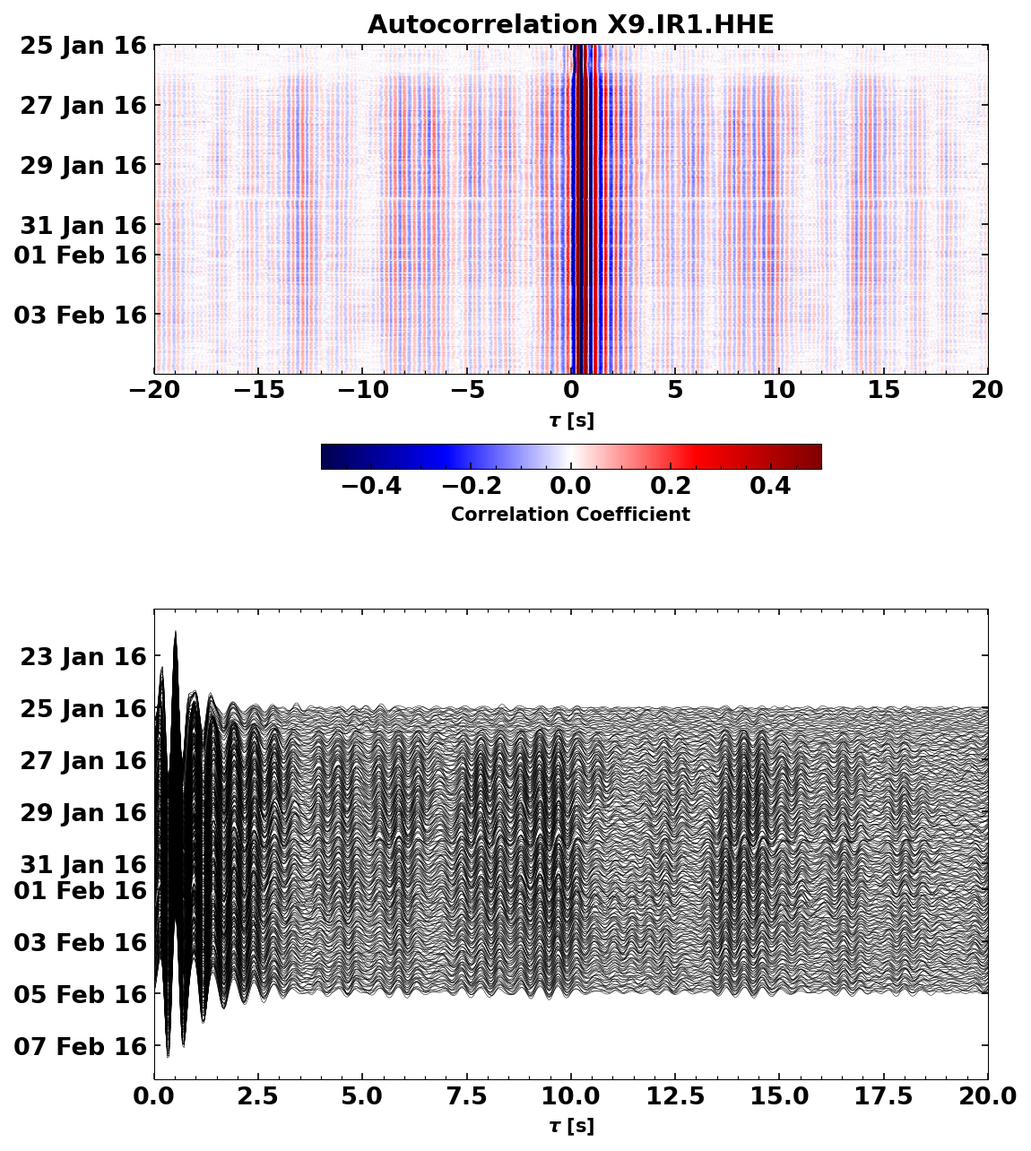
If you look very very closely, you can see a slight time shift in the late coda on January 30th. This time shift is associated to the Zhupanov earthquake. We will try to quantify the velocity change in the following.
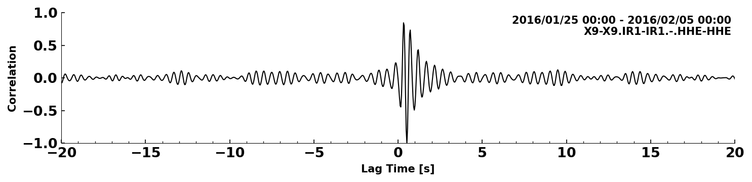
We can also look at a single correlations or at a stack of correlations.
SeisMIC can stack correlation with CorrStream.stack:
corrstack = cst.stack()[0]
corrstack.plot(tlim=[-20,20])
<Axes: xlabel='Lag Time [s]', ylabel='Correlation'>
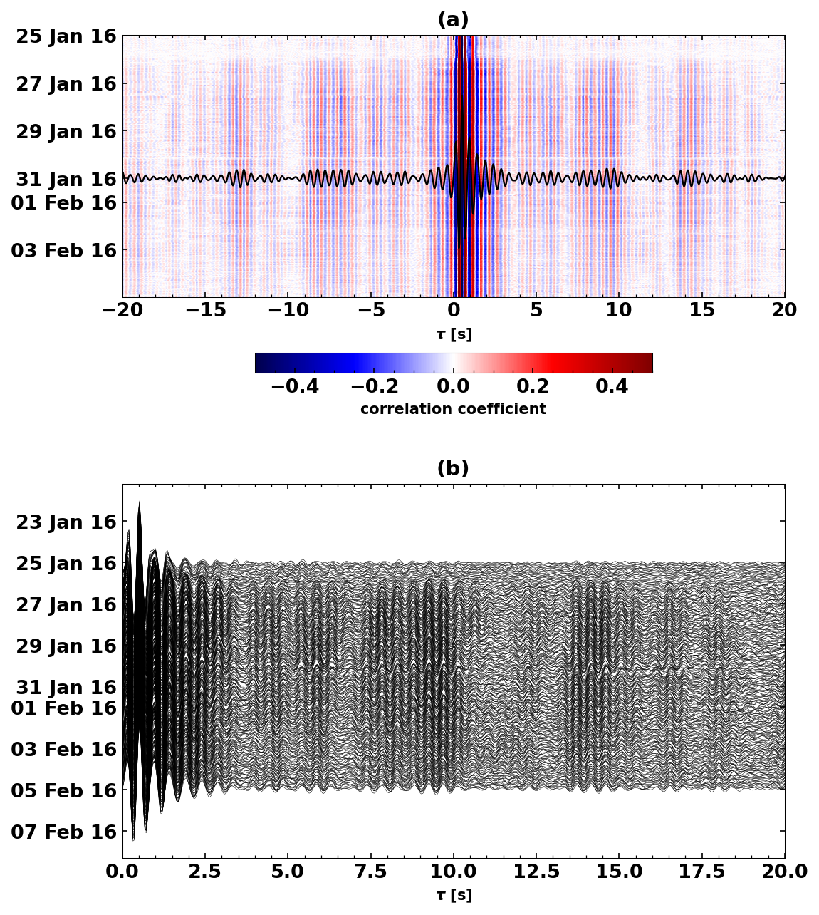
Let’s try and combine the two last plots#
plt.figure(figsize=(8, 10))
ax0 = plt.subplot(2, 1, 1)

cst.plot(timelimits=[-20, 20], cmap='seismic', vmin=-0.5, vmax=0.5, ax=ax0)
ax0.set_title(f'(a)')
ax0.plot(
    corrstack.times(),
    [UTCDateTime(i).datetime for i in corrstack.data*3e5 +  UTCDateTime(2016, 1, 31).timestamp],
    color='k', zorder=100, linewidth=1.1)

ax1 = plt.subplot(2, 1, 2)
cst.plot(scalingfactor=3, timelimits=[0, 20], type='section', ax=ax1)
ax1.set_title(f'(b)')
Text(0.5, 1.0, '(b)')
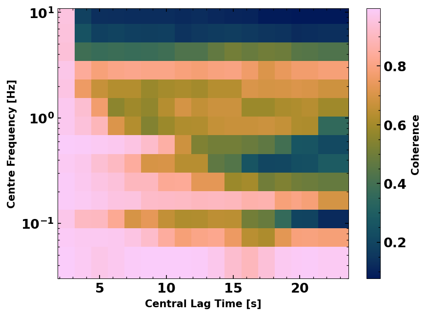
3. Waveform Coherence#
We can assess the average stability of the wavefield in different frequency bands and along the lapse time axis using a measure called the waveform coherence (see ,e.g., Steinmann, et al., 2021). The waveform coherence is the zero lag correlation of two noise correlations. Here we average them for one station and given frequency and lapse time bands.
For this step, we will have to compute a few more noise correlations over various frequency bands. That’s why the next cell will take a while.
!python wfc.py
2023-08-24 10:54:53,301 - WARNING - No existing data found.
Automatically setting preprocess_subdiv to False to optimise performance.
100%|███████████████████████████████████████████| 11/11 [00:05<00:00,  1.92it/s]
2023-08-24 10:54:59,090 - WARNING - No existing data found.
Automatically setting preprocess_subdiv to False to optimise performance.
2023-08-24 10:54:59,090 - WARNING - No existing data found.
Automatically setting preprocess_subdiv to False to optimise performance.
100%|███████████████████████████████████████████| 11/11 [00:05<00:00,  2.02it/s]
2023-08-24 10:55:04,616 - WARNING - No existing data found.
Automatically setting preprocess_subdiv to False to optimise performance.
2023-08-24 10:55:04,616 - WARNING - No existing data found.
Automatically setting preprocess_subdiv to False to optimise performance.
2023-08-24 10:55:04,616 - WARNING - No existing data found.
Automatically setting preprocess_subdiv to False to optimise performance.
100%|███████████████████████████████████████████| 11/11 [00:05<00:00,  2.04it/s]
2023-08-24 10:55:10,090 - WARNING - No existing data found.
Automatically setting preprocess_subdiv to False to optimise performance.
2023-08-24 10:55:10,090 - WARNING - No existing data found.
Automatically setting preprocess_subdiv to False to optimise performance.
2023-08-24 10:55:10,090 - WARNING - No existing data found.
Automatically setting preprocess_subdiv to False to optimise performance.
2023-08-24 10:55:10,090 - WARNING - No existing data found.
Automatically setting preprocess_subdiv to False to optimise performance.
100%|███████████████████████████████████████████| 11/11 [00:05<00:00,  1.96it/s]
2023-08-24 10:55:15,767 - WARNING - No existing data found.
Automatically setting preprocess_subdiv to False to optimise performance.
2023-08-24 10:55:15,767 - WARNING - No existing data found.
Automatically setting preprocess_subdiv to False to optimise performance.
2023-08-24 10:55:15,767 - WARNING - No existing data found.
Automatically setting preprocess_subdiv to False to optimise performance.
2023-08-24 10:55:15,767 - WARNING - No existing data found.
Automatically setting preprocess_subdiv to False to optimise performance.
2023-08-24 10:55:15,767 - WARNING - No existing data found.
Automatically setting preprocess_subdiv to False to optimise performance.
100%|███████████████████████████████████████████| 11/11 [00:05<00:00,  1.97it/s]
2023-08-24 10:55:21,427 - WARNING - No existing data found.
Automatically setting preprocess_subdiv to False to optimise performance.
2023-08-24 10:55:21,427 - WARNING - No existing data found.
Automatically setting preprocess_subdiv to False to optimise performance.
2023-08-24 10:55:21,427 - WARNING - No existing data found.
Automatically setting preprocess_subdiv to False to optimise performance.
2023-08-24 10:55:21,427 - WARNING - No existing data found.
Automatically setting preprocess_subdiv to False to optimise performance.
2023-08-24 10:55:21,427 - WARNING - No existing data found.
Automatically setting preprocess_subdiv to False to optimise performance.
2023-08-24 10:55:21,427 - WARNING - No existing data found.
Automatically setting preprocess_subdiv to False to optimise performance.
100%|███████████████████████████████████████████| 11/11 [00:05<00:00,  1.98it/s]
2023-08-24 10:55:27,068 - WARNING - No existing data found.
Automatically setting preprocess_subdiv to False to optimise performance.
2023-08-24 10:55:27,068 - WARNING - No existing data found.
Automatically setting preprocess_subdiv to False to optimise performance.
2023-08-24 10:55:27,068 - WARNING - No existing data found.
Automatically setting preprocess_subdiv to False to optimise performance.
2023-08-24 10:55:27,068 - WARNING - No existing data found.
Automatically setting preprocess_subdiv to False to optimise performance.
2023-08-24 10:55:27,068 - WARNING - No existing data found.
Automatically setting preprocess_subdiv to False to optimise performance.
2023-08-24 10:55:27,068 - WARNING - No existing data found.
Automatically setting preprocess_subdiv to False to optimise performance.
2023-08-24 10:55:27,068 - WARNING - No existing data found.
Automatically setting preprocess_subdiv to False to optimise performance.
100%|███████████████████████████████████████████| 11/11 [00:05<00:00,  2.00it/s]
100%|█████████████████████████████████████████████| 1/1 [00:00<00:00,  1.12it/s]
100%|█████████████████████████████████████████████| 1/1 [00:00<00:00,  1.11it/s]
100%|█████████████████████████████████████████████| 1/1 [00:00<00:00,  1.07it/s]
100%|█████████████████████████████████████████████| 1/1 [00:00<00:00,  1.05it/s]
100%|█████████████████████████████████████████████| 1/1 [00:00<00:00,  1.07it/s]
100%|█████████████████████████████████████████████| 1/1 [00:00<00:00,  1.06it/s]
100%|█████████████████████████████████████████████| 1/1 [00:00<00:00,  1.07it/s]
from seismic.monitor.wfc import WFCBulk
from seismic.monitor.wfc import read_wfc

wfcs = read_wfc('data/wfc/WFC-X9-X9.IR1-IR1.av.*.npz')
WFCBulk(wfcs).plot(log=True, cmap='batlow')
<Axes: xlabel='Central Lag Time [s]', ylabel='Centre Frequency [Hz]'>
4. Monitoring#
Next, we will compute a velocity change estimate using the stretching
technique (Sens-Schönfelder & Wegler,
2006).
You can find the corresponding parameters in the dv section of the
params.yaml file.
Similarly to the Correlation we can start the monitoring via a simple script:
!cat monitor.py
import os
# This tells numpy to only use one thread
# As we use MPI this is necessary to avoid overascribing threads
os.environ['OPENBLAS_NUM_THREADS'] = '1'

from seismic.monitor.monitor import Monitor

yaml_f = 'params.yaml'
m = Monitor(yaml_f)
m.compute_velocity_change_bulk()
try: ipynb_path
except NameError: ipynb_path = os.getcwd()

os.chdir(ipynb_path)

# multi-core is not necessarily useful for this example
# because the jobs are split into N jobs, where N is the number of
# component combinations (in our case N==1)
ncpus = os.cpu_count()//2
!mpirun -n $ncpus python ./monitor.py
0it [00:00, ?it/s]
0it [00:00, ?it/s]/1 [00:00<?, ?it/s]
0it [00:00, ?it/s]
0it [00:00, ?it/s]
0it [00:00, ?it/s]
saving to X9-X9_IR1-IR1_HHE-HHE
100%|██████████| 1/1 [00:04<00:00,  4.43s/it]
Make a first plot to get an idea of dv/v#
We can use SeisMIC’s inbuilt plotting function for that. The velocity changes will in general be shown in decimal values.
from seismic.monitor.dv import read_dv
dv = read_dv(f'data/vel_change/DV-{network}-{network}.{station}-{station}.HHE-HHE.npz')
dv.plot(ylim=(-0.01,0.01))

# We can print some information about the dv object
print(dv)
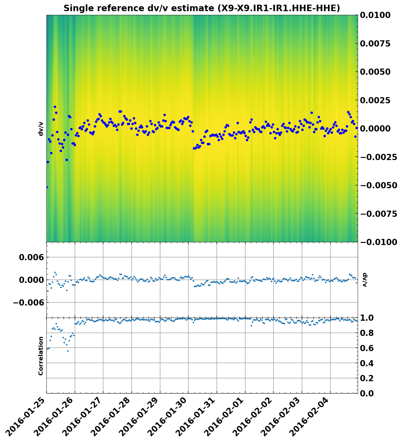
single_ref stretch velocity change estimate of X9-X9.IR1-IR1.HHE-HHE.
starttdate: Mon Jan 25 00:00:00 2016
enddate: Fri Feb  5 00:00:00 2016

processed with the following parameters: {'freq_min': 2.0, 'freq_max': 4.0, 'tw_start': 3.5, 'tw_len': 8.5}
Even with comparably little data, we can see the velocity drop on January 30th. Note that due to the high energy noise, we are able to retrieve a very high resolution estimate of dv/v.
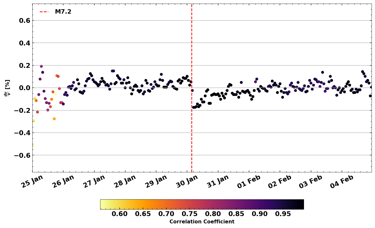
Make the plot look a little nicer#
The plot above is very good if you just want to understand what is going on, but maybe it is not necessarily something you would want to put into a publication. Here is a code that makes the plot look like in the above mentioned publication
from obspy import UTCDateTime

from seismic.plot.plot_utils import set_mpl_params

set_mpl_params()

# Origin Time of the Zhupanov earthquake
otime = UTCDateTime(2016, 1, 30, 3, 25).datetime

fig, ax = dv.plot(style='publication', return_ax=True, ylim=(-.75,.75),
                  dateformat='%d %b')

plt.axvline(otime, linestyle='dashed', c='r', label='M7.2')
plt.legend()
<matplotlib.legend.Legend at 0x7f6293a57730>
What comes next?#
Increasing the stability#
In this case, we are fortunate enough to receive a high-resolution
dv/v estimate with the given parameters (not quite by coincidence
;-)).
For many other datasets, you might not be able to achieve satisfactory
stability. Here are some suggestions on how you could tackle that: 1.
Increase the smoothing. This can be done over a number of different
ways, all of them can be configured in params.yaml: - increase
dv['win_len'] to stack correlations over the defined amount of time
(in seconds) - in dv['preprocessing'] increase the parameter
wsize of the smooth function to smoooth the correlation
functions over a larger amount of time (see
documentation)
- In dv['postprocessing'] set a smoothing of the similarity matrix
(see
documentation)
2. Try different frequencies, different lag time windows of the coda or
a different preprocessing. 3. Stack the results from several component
combinations as done in Illien et
al. 2023.
The corresponding function in Seismic is in
seismic.monitor.monitor.average_component_combinations()
Explore other processing possibilities#
There are a large number of flavours for different processing options
explored. Some of which are natively shipped in SeisMIC. You can
experiment with options to processing your noise correlation functions
differently or compute dv/v differently (e.g., thinking about other
algorithms than the stretching technique). By the way: the dictionaries
in the different processing parameters in params.yaml allow to
import external functions as long as they are scripted in the right way
(see link).
Invert for a velocity change map#
The module seismic.monitor.spatial implements the surface wave
spatial inversion as proposed by Obermann et
al. (2013).
Consult the documentation, to learn how to work with spatial inversions.
You can continue with the spatial Jupyter Notebook
to learn how to do a spatial inversion with SeisMIC.
References#
List of references used in this notebook.
Download this notebook#
You can download this notebook on our GitHub page