%%{init: { 'logLevel': 'debug', 'theme': 'base' } }%%
graph LR
    waveform[Get Data] --> correlate(Correlation)
    correlate:::active -->|save| corrdb[(CorrDB/hdf5)]
    corrdb --> monitor
    monitor[Measure dv] -->|save| dv{{DV}}
    click waveform "../trace_data.html" "trace_data"
    click correlate "../correlate.html" "correlate"
    click monitor "../monitor.html" "monitor"
    click corrdb "../corrdb.html" "CorrDB"
    click dv "../monitor/dv.html" "DV"
    classDef active fill:#f666, stroke-width:4px, stroke:#f06;
    

CorrTrace, CorrStream, and CorrBulk classes

Once the correlations are actually computed, they are assigned as CorrTrace and CorrStream objects. Both inherit most of their methods and attributes from their obspy parents. However, there are some extra attributes and functionalities.

CorrTrace

Most notably a new Header object (CorrStats) with different attributes is associated to this type of trace. The header takes care of saving vital information like lag times (start_lag and end_lag), the start- and the endtime of the waveforms that were used to compute the correlation (corr_start and corr_end, respectively), and information about the coordinates of the stations.

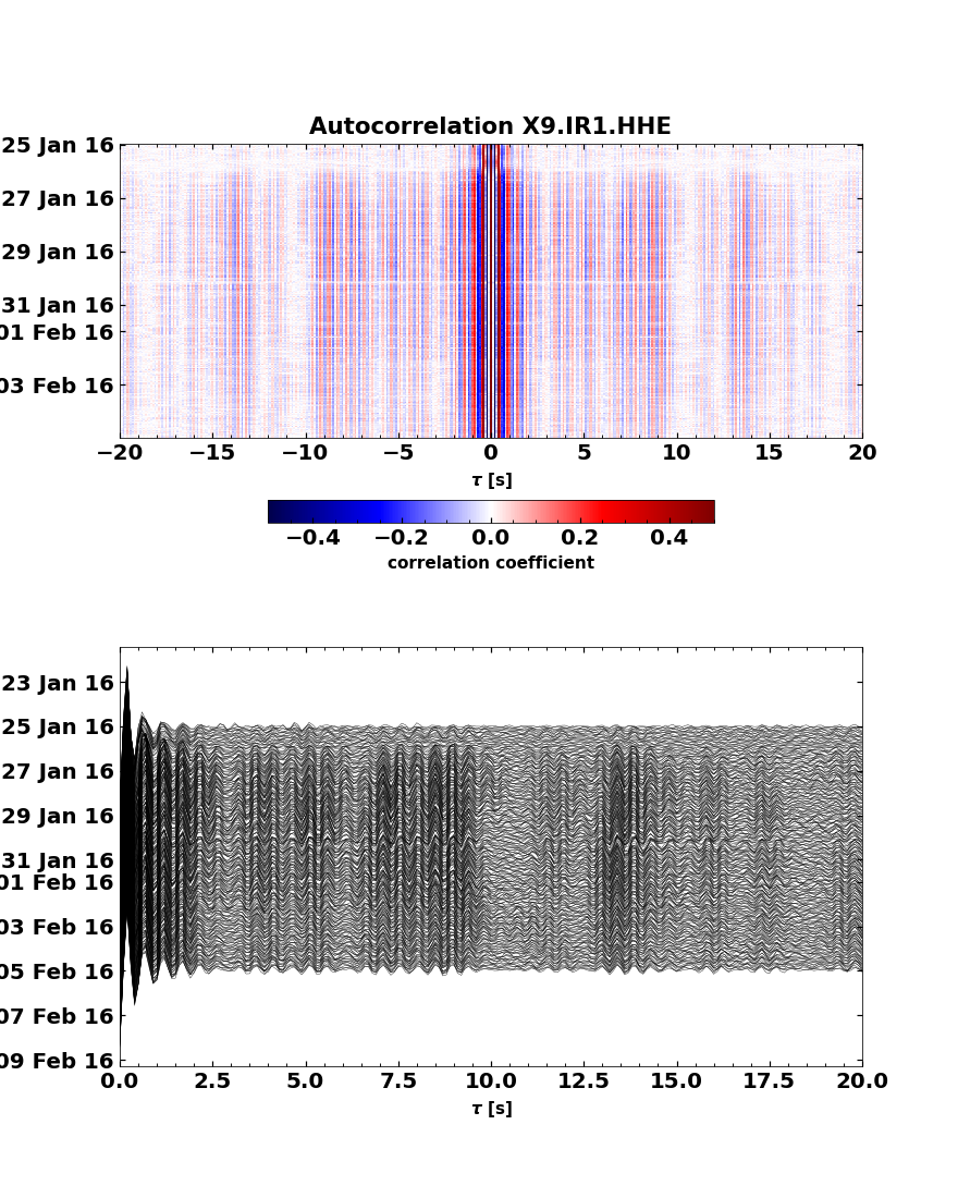
CorrTrace does also come with its own plotting method plot() (check it for details). It can produce plots akin to this one:

CorrStream

Essentially, this class is just a fancy list of CorrTrace objects. However, it has methods to stack (stack()), select (select_corr_time()), or slide (slide()) time windows. It also enables us to create section stacks, sorted by interstation distance or time:

CorrBulk

CorrStream does also have a method to create a CorrBulk object (create_corr_bulk()). Instead of relying on a list of traces, this object is based on numpy arrays, which makes all sorts of computations cheaper. Check out CorrBulk for available functions. This is also the object that SeisMIC’s own monitoring workflow is based on.